Normal & Non-normal Distributions

Many analytical techniques assume normality

Normal Distribution (Gaussian Distribution)

A normal distribution is a symmetric, bell-shaped probability distribution defined by its mean (μ) and standard deviation (σ).

Key Characteristics:

• Symmetry: Mean = Median = Mode

• Bell-shaped curve

• Data is evenly distributed around the center

• Predictable variability using standard deviation

• Empirical Rule (68–95–99.7):

  • 68% of data within ±1σ

  • 95% within ±2σ

  • 99.7% within ±3σ

Why It Matters:

Normal distribution allows the use of parametric statistical methods, which are more powerful and efficient. These include:

• Hypothesis testing (t-tests, ANOVA)

• Regression analysis

• Process capability indices (Cp, Cpk)

Non-Normal Distribution

Any distribution that does not follow the normal pattern is considered non-normal.

Common Types:

a) Skewed Distributions

• Positive skew (right-skewed): tail extends right

• Negative skew (left-skewed): tail extends left

b) Uniform Distribution

• All values have equal probability

c) Exponential Distribution

• Models time between events

d) Bimodal / Multimodal

• More than one peak

Why This Distinction is Critical

In high maturity environments (e.g., CMMI Level 4 & 5), organizations rely on:

• Process Performance Baselines (PPBs)

• Process Performance Models (PPMs)

If the underlying data is non-normal:

• Capability indices (Cp, Cpk) may be invalid

• Predictions may be inaccurate

• Process behavior may be misunderstood

Normality Test

Normality tests evaluate whether a dataset significantly deviates from a normal (Gaussian) distribution.

• Null Hypothesis (H₀): Data is normally distributed

• Alternative Hypothesis (H₁): Data is not normally distributed

If the p-value < 0.05, you typically reject normality.

Choosing the Right Test

Small sample (<50) ---> Shapiro–Wilk

Medium sample (50–2000)---> Shapiro–Wilk / Anderson–Darling

Large sample (>2000)---> Anderson–Darling / Jarque–Bera

Tail-sensitive analysis---> Anderson–Darling

What If Data Is Not Normal?

Transform the Data

• Log transformation

• Box-Cox transformation

Use Non-Parametric Methods

• Mann–Whitney U Test

• Kruskal–Wallis Test

Apply Distribution-Specific Models

• Weibull (reliability)

• Exponential (failure rates)

Key Normality Tests

1. Shapiro–Wilk Test (Most Recommended)

• Best for small to medium samples (n < 2000)

• High statistical power (detects deviations effectively)

Use Case: General-purpose normality validation in most business datasets

2. Kolmogorov–Smirnov (K–S) Test

• Compares sample distribution with a reference normal distribution

• Less powerful than Shapiro–Wilk

Limitation: Sensitive to sample size and distribution parameters

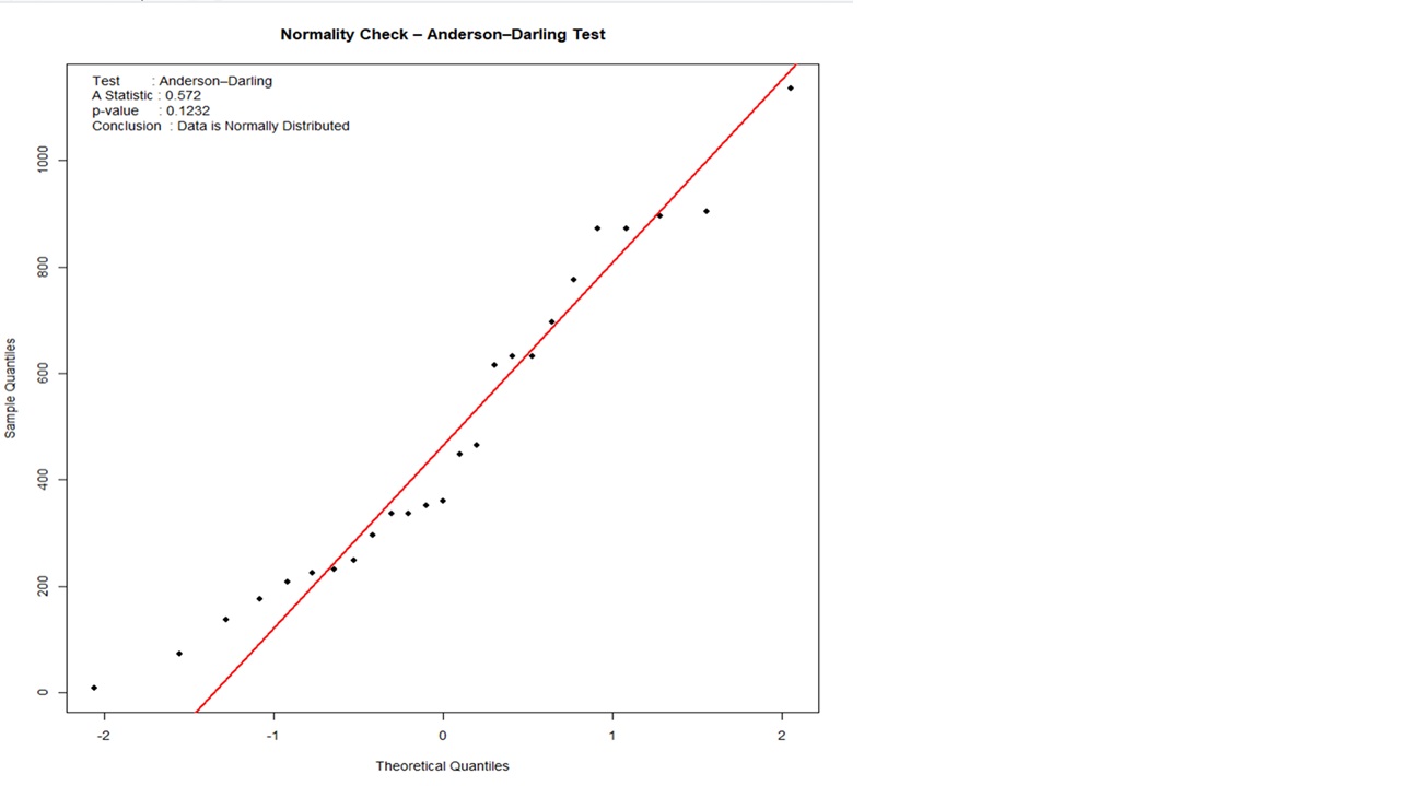
3. Anderson–Darling Test

• Focuses more on tail behaviour (important for risk analysis)

• More sensitive than K–S

Use Case: Quality control, reliability, defect analysis

Graphical Methods (Always Use Alongside Tests)

Statistical tests alone can mislead—visual validation is essential.

Histogram

• Look for symmetry and bell shape

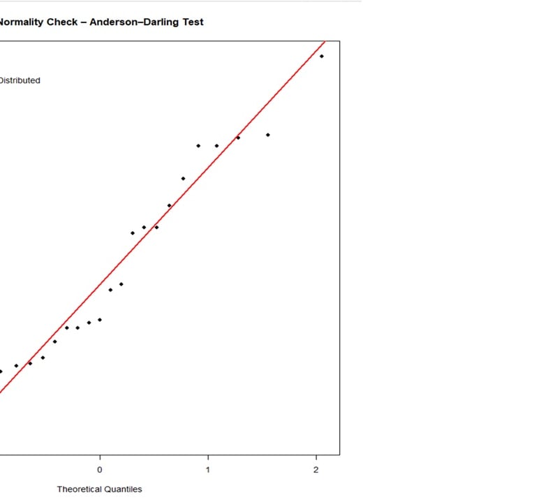
Q-Q Plot (Quantile–Quantile Plot)

• Points should align along a straight diagonal

Box Plot

• Identifies skewness and outliers

Key Normality Tests